The Guide to DeepLearning with Tensorflow and Keras - The Beginning

Learn how to build a neural network and how to train, evaluate and optimize it with TensorFlow.

This is a part-by-part course which we will cover from basics to implementing models in productions.


Today’s TensorFlow tutorial for beginners will introduce you to performing deep learning in an interactive way:


You’ll first learn more about tensors;

Then, the tutorial you’ll briefly go over some of the ways that you can install TensorFlow on your system so that you’re able to get started and load data in your workspace;

After this, you’ll go over some of the TensorFlow basics: you’ll see how you can easily get started with simple computations.




What is TensorFlow?

TensorFlow is a popular open source library that's used for implementing machine learning and deep learning.

It was initially built at Google for internal consumption and was released publicly on November 9, 2015.

Since then, TensorFlow has been extensively used to develop machine learning and deep learning models in several business domains.



To use TensorFlow in our projects, we need to learn how to program using the TensorFlow API. 


TensorFlow has multiple APIs that can be used to interact with the library. The TensorFlow APIs are divided into two levels:



Low-level API: The API known as TensorFlow core provides fine-grained lower level functionality. Because of this, this low-level API offers complete control while being used on models. We will cover TensorFlow core in this post.



High-level API: These APIs provide high-level functionalities that have been built on TensorFlow core and are comparatively easier to learn and implement. Some high-level APIs include Estimators, Keras, TFLearn, TFSlim, and Sonnet.


The TensorFlow core

The TensorFlow core is the lower-level API on which the higher-level TensorFlow modules are built. In this section, 


We will go over a quick overview of TensorFlow core and learn about the basic elements of TensorFlow.


Here we go! Let’s begin the fundamentals of Tensorflow.🙏🙏


Setting up Tensorflow.

TensorFlow is tested and supported on the following 64-bit systems:

• Ubuntu 16.04 or later
• Windows 7 or later
• macOS 10.12.6 (Sierra) or later (no GPU support)
• Raspbian 9.0 or later

##### Current release for CPU-only
pip install tensorflow

##### Nightly build for CPU-only (unstable)
pip install tf-nightly

##### GPU package for CUDA-enabled GPU cards
pip install tensorflow-gpu

##### Nightly build with GPU support (unstable)
pip install tf-nightly-gpu

Lets Spice things with Hello World! Example!

import tensorflow as tf
hello = tf.constant("hello wold")
sess = tf.Session()
print(sess.run(hello))
print('--------------')
--------------------
b'hello wold'
--------------

We will check line by line what we have written and how we implemented out Hello World! example

Tensorflow fundamentals.

First, we’re going to take a look at the tensor object type. Then we’ll have a graphical understanding of TensorFlow to define computations. Finally,

we’ll run the graphs with sessions, showing how to substitute intermediate values.


Tensors


Tensors are the basic components in TensorFlow. A tensor is a multidimensional collection of data elements.



It is generally identified by shape, type, and rank. Rank refers to the number of dimensions of a tensor, while shape refers to the size of each dimension.



You may have seen several examples of tensors before, such as in a zero-dimensional collection (also known as a scalar), a one-dimensional collection (also known as a vector), and a two-dimensional collection (also known as a matrix).





A scalar value is a tensor of rank 0 and shape []. A vector, or a one-dimensional array, is a tensor of rank 1 and shape [number_of_columns] or [number_of_rows]

Let's create some constants with the following code:

const1=tf.constant(34,name='x1')
const2=tf.constant(59.0,name='y1')
const3=tf.constant(32.0,dtype=tf.float16,name='z1')

print('const1 (x): ',const1)
print('const2 (y): ',const2)
print('const3 (z): ',const3)

Let's take a look at the preceding code in detail:

• The first line of code defines a constant tensor, const1, stores a value of 34, and names it x1.
• The second line of code defines a constant tensor, const2, stores a value of 59.0, and names it y1.
• The third line of code defines the data type as tf.float16 for const3. Use the dtype parameter or place the data type as the second argument to denote the data type. 

Example:

hello = tf.constant("Hello ")
world = tf.constant("World")
type(hello)
print(hello)


with tf.Session() as sess:
    result = sess.run(hello+world)
    
    
print(result)

--------------------
tensorflow.python.framework.ops.Tensor
Tensor("Const_1:0", shape=(), dtype=string)
b'Hello World'

Constants

The constant valued tensors are created using the tf.constant() function, and has the following definition:

Syntax:

tf.constant(
  value,
  dtype=None,
  shape=None,
  name='const_name',
  verify_shape=False
  )

Let's create some constants with the following code:

a = tf.constant(10)
b = tf.constant(20)

const1=tf.constant(34,name='x1')
const2=tf.constant(59.0,name='y1')
const3=tf.constant(32.0,dtype=tf.float16,name='z1')

print(a)
print(b)
print('const1 (x): ',const1)
print('const2 (y): ',const2)
print('const3 (z): ',const3)
------------------------------
Tensor("Const_1:0", shape=(), dtype=int32)
Tensor("Const_2:0", shape=(), dtype=int32)
const1 (x):  Tensor("x:0", shape=(), dtype=int32)
const2 (y):  Tensor("y:0", shape=(), dtype=float32)
const3 (z):  Tensor("z:0", shape=(), dtype=float16)

Operations

How can we do addition/multiplication in tensorflow ?.



The TensorFlow library contains several built-in operations that can be applied on tensors. 



An operation node can be defined by passing input values and saving the output in another tensor. To understand this better, let's define two operations.

a = tf.constant(10)
b = tf.constant(20)
type(a)

with tf.Session() as sess:
    result = sess.run(a+b)
    mul = sess.run(tf.multiply(a,b))
    
print(result)
print(mul)
------------------
30
200

Some of the built-in operations of TensorFlow include arithmetic operations, math functions, and complex number operations.



Working with Matrices in Tensorflow.


We can easily create n*n matrices in tensorflow using the in-built functions. We' ll dicrectly dive into the example to understand the code.

const = tf.constant(10)



## Building a 4*4 Matix with all element as 10
## We are going to use fill() to fill the matrix with default value
## fill((row,col),def_value) can be used to fill values.
fill_mat = tf.fill((4,4),10)


## Creating a zero 4*4 Matrix
## Default tr.zeros() to create a zero matrix
myzeros = tf.zeros((4,4))


## Creating one matrices
## Using tf.one() method to create one matrix

myones = tf.ones((4,4))

## Creating a random normalized matrix.
## Using random_normal Outputs random values from a normal distribution.
## mean: A 0-D Tensor or Python value of type dtype. stddev: A 0-D Tensor or Python value of type dtype.

myrand = tf.random_normal((4,4),mean =0,stddev =1.0)

myrandu = tf.random_uniform((4,4),minval=0,maxval=1)

my_ops = [const,fill_mat,myzeros,myones,myrand,myrandu]

sess = tf.InteractiveSession()


for op in my_ops:
print(sess.run(op))
print("\n")

--------------------------------------------------
10


[[10 10 10 10]
[10 10 10 10]
[10 10 10 10]
[10 10 10 10]]


[[0. 0. 0. 0.]
[0. 0. 0. 0.]
[0. 0. 0. 0.]
[0. 0. 0. 0.]]


[[1. 1. 1. 1.]
[1. 1. 1. 1.]
[1. 1. 1. 1.]
[1. 1. 1. 1.]]


[[-1.1485276 0.6817215 1.6923033 1.0417686 ]
[ 0.75727195 -0.6906906 1.382049 0.26310864]
[-1.3289255 -2.0204604 0.9086128 -1.6753776 ]
[ 0.83860254 0.8221855 -0.01571688 0.33962643]]


[[0.4758848 0.02705026 0.45411873 0.9472964 ]
[0.03372979 0.04275322 0.51311064 0.1727488 ]
[0.38706803 0.29606903 0.17789984 0.97908235]
[0.2033397 0.9660599 0.6367506 0.9244758 ]]

Placeholders

While constants store the value at the time of defining the tensor, placeholders allow you to create empty tensors so that the values can be provided at runtime. 



The TensorFlow library provides the tf.placeholder() function with the following signature to create placeholders:

Syntax:

tf.placeholder(
  dtype,
  shape=None,
  name=None
  )

Lets see with an example

p1 = tf.placeholder(tf.float32)
p2 = tf.placeholder(tf.float32)
print('p1 : ', p1)
print('p2 : ', p2)

--------------------
p1 :  Tensor("Placeholder:0", dtype=float32)
p2 :  Tensor("Placeholder_1:0", dtype=float32)

Computation graph/Tensorflow Graph

A computation graph is the basic unit of computation in TensorFlow. A computation graph consists of nodes and edges. Each node represents an instance of tf.Operation,

while each edge represents an instance of tf.Tensor that gets transferred between the nodes.

A model in TensorFlow contains a computation graph. First, you must create the graph with the nodes representing variables, constants, placeholders, and operations, and then provide the graph to the TensorFlow execution engine.



 The TensorFlow execution engine finds the first set of nodes that it can execute. The execution of these nodes starts the execution of the nodes that follow the sequence of the computation graph.

Thus, TensorFlow-based programs are made up of performing two types of activities on computation graphs:

• Defining the computation graph
• Executing the computation graph

A TensorFlow program starts execution with a default graph. Unless another graph is explicitly specified, a new node gets implicitly added to the default graph. Explicit access to the default graph can be obtained using the following command:

graph = tf.get_default_graph()

n1 = tf.constant(1)
n2 = tf.constant(2)
n3 =n1+n2
with tf.Session() as sess:
    result = sess.run(n3)
 
result
print(tf.get_default_graph())
g =tf.Graph()
print(g)
graph_one = tf.get_default_graph()
print(graph_one)
graph_two = tf.Graph()
with graph_two.as_default():
    print(graph_two is tf.get_default_graph())
--------------------------------------

<tensorflow.python.framework.ops.Graph object at 0x0000022C46285CF8>
<tensorflow.python.framework.ops.Graph object at 0x0000022C47F8D390>
<tensorflow.python.framework.ops.Graph object at 0x0000022C46285CF8>

True

`


Here are the advantages of organizing the computations as a graph,

• Parallelism. By using explicit edges to represent dependencies between operations, it is easy for the system to identify operations that can execute in parallel.
• Distributed execution. By using explicit edges to represent the values that flow between operations, it is possible for TensorFlow to partition your program across multiple devices (CPUs, GPUs, and TPUs) attached to different machines.
• TensorFlow inserts the necessary communication and coordination between devices.
• Compilation. TensorFlow’s XLA compiler can use the information in your dataflow graph to generate faster code, for example, by fusing together adjacent operations.

Session

We have seen in all the earlier example of running our tensorflow graph into a tensorflow session.


TensorFlow uses tf.Session class to represent a connection between the client program---typically a Python program, although a similar interface is available in other languages---and the C++ runtime. 


A tf.Session object provides access to devices in the local machine, and remote devices using the distributed TensorFlow runtime. It also caches information about your tf.Graph so that you can efficiently run the same computation multiple times.

Syntax:

# Creating a tf.Session
If you are using the low-level TensorFlow API, you can create a tf.Session for the current default graph as follows:

# Create a default in-process session.
with tf.Session() as sess:
  # ...

# Create a remote session.
with tf.Session("grpc://example.org:2222"):
  # ...

Since a tf.Session owns physical resources (such as GPUs and network connections), it is typically used as a context manager (in a with block) that automatically closes the session 


when you exit the block. It is also possible to create a session without using a with a block, but you should explicitly call tf.Session.close when you are finished with it to free the resources.

That's all for the starting I hope you can start practicing Tensorflow along with me and we can deep dive and start exploring more about it soon.


We’ll be back with more exciting discussions not just on building Deep learning models but also on building a robust infrastructure to store, consume and process data at scale.


 Till then, happy coding!💓💓

A Deep Intro to Machine Learning(Python) - A Beginners Guide

Welcome to the world of machine learning with scikit-learn. Machine learning can be overwhelming at times and this is partly due to a large number of tools that are available on the market. This post will simplify this process of tool selection down to one – scikit-learn. 

In this Series, you will learn how to construct an end-to-end machine learning pipeline using some of the most popular algorithms that are widely used in industry and professional competitions, such as Kaggle. 

However, in this introductory post, we will go through the following topics:

• A brief introduction to machine learning
• What is scikit-learn?
• Installing scikit-learn
• Algorithms that you will learn to implement scikit-learn in series.
• Example to build your first regression model

Now, let's begin this fun journey into the world of machine learning with scikit-learn!

A brief introduction to machine learning!

Machine learning has generated quite the buzz – from Elon Musk fearing the role of unregulated artificial intelligence in society, to Mark Zuckerberg having a view that contradicts Musk. 💥

So, what exactly is machine learning? Simply put, machine learning is a set of methods that can detect patterns in data and use those patterns to make future predictions. Machine learning has found immense value in a wide range of industries, ranging from finance to healthcare. This translates to a higher requirement of talent with the skill capital in the field of machine learning.

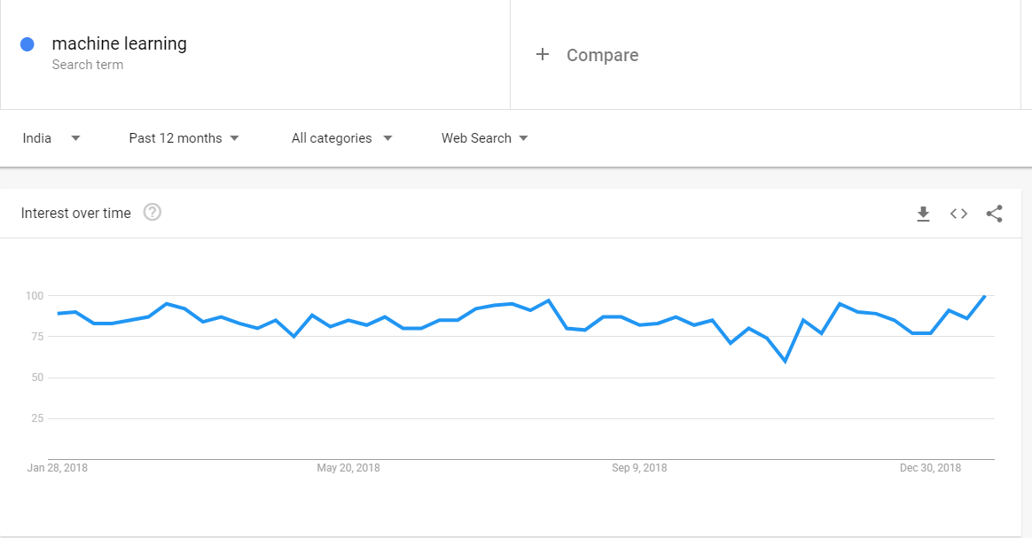
Here is a quick Overview of google trend for machine learning.😧

Broadly speaking, machine learning can be categorized into three main types:

• Supervised learning
• Unsupervised learning
• Reinforcement learning

Supervised learning

Supervised learning is a form of machine learning in which our data comes with a set of labels or a target variable that is numeric. These labels/categories usually belong to one feature/attribute, which is commonly known as the target variable. For instance, each row of your data could either belong to the category of Healthy or Not Healthy.

Given a set of features such as weight, blood sugar levels, and age, we can use the supervised machine learning algorithm to predict whether the person is healthy or not. 

In the following simple mathematical expression, S is the supervised learning algorithm, X is the set of input features, such as weight and age, and Y is the target variable with the labels Healthy or Not Healthy:

Although supervised machine learning is the most common type of machine learning that is implemented with scikit-learn and in the industry, most datasets typically do not come with predefined labels. Unsupervised learning algorithms are first used to cluster data without labels into distinct groups to which we can then assign labels. This is discussed in detail in the following section.

Supervised learning algorithms

Supervised learning algorithms can be used to solve both classification and regression problems.  you will learn how to implement some of the most popular supervised machine learning algorithms. Popular supervised machine learning algorithms are the ones that are widely used in industry and research, and have helped us solve a wide range of problems across a wide range of domains. These are some of supervised learning algorithms are as follows:

• Linear regression: This supervised learning algorithm is used to predict continuous numeric outcomes such as house prices, stock prices, and temperature, to name a few
• Logistic regression: The logistic learning algorithm is a popular classification algorithm that is especially used in the credit industry in order to predict loan defaults
• k-Nearest Neighbors: The k-NN algorithm is a classification algorithm that is used to classify data into two or more categories, and is widely used to classify houses into expensive and affordable categories based on price, area, bedrooms, and a whole range of other features
• Support vector machines: The SVM algorithm is a popular classification algorithm that is used in image and face detection, along with applications such as handwriting recognition
• Tree-Based algorithms: Tree-based algorithms such as decision trees, Random Forests, and Boosted trees are used to solve both classification and regression problems
• Naive Bayes: The Naive Bayes classifier is a machine learning algorithm that uses the mathematical model of probability to solve classification problems

Unsupervised learning

Unsupervised learning is a form of machine learning in which the algorithm tries to detect/find patterns in data that do not have an outcome/target variable. In other words, we do not have data that comes with pre-existing labels. Thus, the algorithm will typically use a metric such as distance to group data together depending on how close they are to each other. 

As discussed in the previous section, most of the data that you will encounter in the real world will not come with a set of predefined labels and, as such, will only have a set of input features without a target attribute. 

In the following simple mathematical expression, U is the unsupervised learning algorithm, while X is a set of input features, such as weight and age:

Given this data, our objective is to create groups that could potentially be labeled as Healthy or Not Healthy. The unsupervised learning algorithm will use a metric such as distance in order to identify how close a set of points are to each other and how far apart two such groups are. 

Unsupervised learning algorithms

Unsupervised machine learning algorithms are typically used to cluster points of data based on distance. The unsupervised learning algorithm that you will learn is as follows:

• k-means: The k-means algorithm is a popular algorithm that is typically used to segment customers into unique categories based on a variety of features, such as their spending habits. This algorithm is also used to segment houses into categories based on their features, such as price and area. 

Reinforcement learning

Reinforcement learning is an area of Machine Learning. Reinforcement. It is about taking suitable action to maximize reward in a particular situation. It is employed by various software and machines to find the best possible behavior or path it should take in a specific situation. Reinforcement learning differs from the supervised learning in a way that in supervised learning the training data has the answer key with it so the model is trained with the correct answer itself whereas in reinforcement learning, there is no answer but the reinforcement agent decides what to do to perform the given task. In the absence of training dataset, it is bound to learn from its experience.

Pre-requisite for the Machine learning (Must Read🙏):

1.  How to Setup Jupyter Notebook perfectly for Data Analysis
2. . Pandas in Python for Data Analysis with Example(Step-by-Step guide)
3.  Data Visualization

Lets Deep Dive In!!

How we are going to do it? 

-- Scikit-learn

Scikit-learn is a free and open source software that helps you tackle supervised and unsupervised machine learning problems. The software is built entirely in Python and utilizes some of the most popular libraries that Python has to offer, namely NumPy and SciPy. 

The main reason why scikit-learn is very popular stems from the fact that most of the world's most popular machine learning algorithms can be implemented quite quickly in a plug and play format once you know what the core pipeline is like. Another reason is that popular algorithms for classification such as logistic regression and support vector machines are written in Cython. Cython is used to give these algorithms C-like performance and thus makes the use of scikit-learn quite efficient in the process. 

Scikit-learn is designed to tackle problems pertaining to supervised and unsupervised learning only and does not support reinforcement learning at present. 

Installing the Scikit- learn package

There are two ways in which you can install scikit-learn on your personal device:

• By using the pip method
• By using the Anaconda method

The pip method can be implemented on the macOS/Linux Terminal or the Windows PowerShell, while the Anaconda method will work with the Anaconda prompt.

Choosing between these two methods of installation is pretty straightforward:

The pip method

pip3 install NumPy
pip3 install SciPy
pip3 install scikit-learn
pip3 install -U scikit-learn

The Anaconda method

conda install NumPy
conda install SciPy
conda install scikit-learn
conda install -U scikit-learn

So far, this lesson has focused on the brief introduction into what machine learning is for those 

of you who are just beginning your journey into the world of machine learning.

You have learned about how scikit-learn fits into the context of machine learning

and how you can go about installing the necessary software.

Now, we'll put this into practice💪 and do some data exploration and analysis.

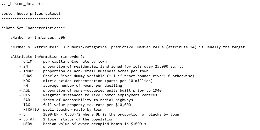
The dataset we'll look at in this section is the so-called Boston housing dataset.

Loading the Data into Jupyter Using a Pandas DataFrame

Often times, data is stored in tables, which means it can be saved as a comma-separated 

variable (CSV) file. This format, and many others can be read into Python as a DataFrame

object, using the Pandas library. Other common formats include tab-separated variable 

(TSV), SQL tables, and JSON data structures. Indeed, Pandas has support for all of these. 

In this example, however, we are not going to load the data this way because of the dataset 

is available directly through scikit-learn.

The Boston housing dataset can be accessed from the module sklearn.datasets using the method.load_boston

from sklearn import datasets
boston = datasets.load_boston()
type(boston)

print(boston['DESCR'])

import pandas as pd

## Loading the data as Dataframe in pandas

df = pd.DataFrame(data=boston['data'], columns = boston['feature_names'])

#Checking our top 5 rows of the dataframe

df.head()

	CRIM	ZN	INDUS	CHAS	NOX	RM	AGE	DIS	RAD	TAX	PTRATIO	B	LSTAT
0	0.00632	18.0	2.31	0.0	0.538	6.575	65.2	4.0900	1.0	296.0	15.3	396.90	4.98
1	0.02731	0.0	7.07	0.0	0.469	6.421	78.9	4.9671	2.0	242.0	17.8	396.90	9.14
2	0.02729	0.0	7.07	0.0	0.469	7.185	61.1	4.9671	2.0	242.0	17.8	392.83	4.03
3	0.03237	0.0	2.18	0.0	0.458	6.998	45.8	6.0622	3.0	222.0	18.7	394.63	2.94
4	0.06905	0.0	2.18	0.0	0.458	7.147	54.2	6.0622	3.0	222.0	18.7	396.90	5.33

In machine learning, the variable that is being modeled is called the target variable; it's what you are trying to predict given the features. For this dataset, the suggested target is MEDV, the median house value in 1,000s of dollars.

## Adding Target temp Column to our dataframe
df['MEDV'] = boston['target']


## Creating copy of the target Value
y = df['MEDV'].copy()

##Deleting the Newly created column
del df['MEDV']


## Concat the target columns to our existing dataframe
df = pd.concat((y, df), axis=1)

	MEDV	CRIM	ZN	INDUS	CHAS	NOX	RM	AGE	DIS	RAD	TAX	PTRATIO	B	LSTAT
0	24.0	0.00632	18.0	2.31	0.0	0.538	6.575	65.2	4.0900	1.0	296.0	15.3	396.9	4.98
1	21.6	0.02731	0.0	7.07	0.0	0.469	6.421	78.9	4.9671	2.0	242.0	17.8	396.9	9.14

Here, we introduce a dummy variable y to hold a copy of the target column before removing it from the DataFrame. We then use the Pandas concatenation function to combine it with the remaining DataFrame along the 1st axis (as opposed to the 0th axis, which combines rows).

print(df.shape)

df.isnull().sum()
---------------------
(506, 14)

MEDV       0
CRIM       0
ZN         0
INDUS      0
CHAS       0
NOX        0
RM         0
AGE        0
DIS        0
RAD        0
TAX        0
PTRATIO    0
B          0
LSTAT      0
dtype: int64

For this dataset, we see there are no NaNs, which means we have no immediate work to do in cleaning the data and can move on.

To simplify the analysis, the final thing we'll do before exploration is remove some of the columns. We won't bother looking at these, and instead focus on the remainder in more detail.
Remove some columns by running the cell that contains the following code:

for col in ['ZN', 'NOX', 'RAD', 'PTRATIO', 'B']:
    del df[col]

Data Exploration

Since this is an entirely new dataset that we've never seen before, the first goal here is to understand the data. We've already seen the textual description of the data, which is important for qualitative understanding. We'll now compute a quantitative description.

 df.describe().T 

count	mean	std	min	25%	50%	75%	max
MEDV	506.0	22.532806	9.197104	5.00000	17.025000	21.20000	25.000000	50.0000
CRIM	506.0	3.613524	8.601545	0.00632	0.082045	0.25651	3.677083	88.9762
INDUS	506.0	11.136779	6.860353	0.46000	5.190000	9.69000	18.100000	27.7400
CHAS	506.0	0.069170	0.253994	0.00000	0.000000	0.00000	0.000000	1.0000
RM	506.0	6.284634	0.702617	3.56100	5.885500	6.20850	6.623500	8.7800
AGE	506.0	68.574901	28.148861	2.90000	45.025000	77.50000	94.075000	100.0000
DIS	506.0	3.795043	2.105710	1.12960	2.100175	3.20745	5.188425	12.1265
TAX	506.0	408.237154	168.537116	187.00000	279.000000	330.00000	666.000000	711.0000
LSTAT	506.0	12.653063	7.141062	1.73000	6.950000	11.36000	16.955000	37.9700

This computes various properties including the mean, standard deviation, minimum, and maximum for each column. This table gives a high-level idea of how everything is distributed. Note that we have taken the transform of the result by adding a .T to the output; this swaps the rows and columns.

cols = ['RM', 'AGE', 'TAX', 'LSTAT', 'MEDV'] 

df[cols].corr()

import matplotlib.pyplot as plt 

import seaborn as sns 
%matplotlib inline 
ax = sns.heatmap(df[cols].corr(), 
                 cmap=sns.cubehelix_palette(20, light=0.95, dark=0.15))
ax.xaxis.tick_top() # move labels to the top

We call sns.heatmap and pass the pairwise correlation matrix as input. We use a custom color palette here to override the Seaborn default.

This resulting table shows the correlation score between each set of values. Large positive scores indicate a strong positive (that is, in the same direction) correlation. As expected, we see maximum values of 1 on the diagonal.

Pearson coefficient is defined as the covariance between two variables, divided by the product of their standard deviations:

The covariance, in turn, is defined as follows:

Here, n is the number of samples, xi and yi are the individual samples being summed over, and Xbar and Ybar are the means of each set.


Linear Model with Scikit-Learn

We can see that it presents us with a regression problem where we predict a continuous target variable given a set of features. In particular, we'll be predicting the median house value (MEDV). We'll train models that take only one feature as input to make this prediction. This way, the models will be conceptually simple to understand and we can focus more on the technical details of the scikit-learn API. 

We'll import the LinearRegression class and build our linear classification model the same way as before, when we calculated the MSE. Run the following:

Use scikit-learn to fit a polynomial regression model to predict the median house value (MEDV), given the LSTAT values. We are hoping to build a model that has a lower mean-squared error (MSE)

y = df['MEDV'].values

x = df['LSTAT'].values.reshape(-1,1)


from sklearn.preprocessing import PolynomialFeatures

poly = PolynomialFeatures(degree=3)

x_poly = poly.fit_transform(x)



from sklearn.linear_model import LinearRegression

clf = LinearRegression()

clf.fit(x_poly, y)


y_pred = clf.predict(x_poly)

resid_MEDV = y - y_pred


from sklearn.metrics import mean_squared_error

error = mean_squared_error(y, y_pred)

print('mse = {:.2f}'.format(error))

fig, ax = plt.subplots()
# Plot the samples
ax.scatter(x.flatten(), y, alpha=0.6)
# Plot the polynomial model
x_ = np.linspace(2, 38, 50).reshape(-1, 1)
x_poly = poly.fit_transform(x_)
y_ = clf.predict(x_poly)
ax.plot(x_, y_, color='red', alpha=0.8)
ax.set_xlabel('LSTAT'); ax.set_ylabel('MEDV');

--------------------------------------
mse = 28.88

This error metric can be converted to an average error in dollars by taking the square root. Doing this for the polynomial model, we find the average error for the median house value is only $5,300.

This completes the extensive guide to understanding how to write your first Machine learning model.

 Here, we used visual assists such as scatter plots,  to deepen our understanding of the data. We also performed simple predictive modeling. In the next part, we will look into what is MSE/RMSE and work with more other models to enhance accuracy.

Hope you liked it! Please Share this guide to other fellow readers. 

Till then Happy Machine learning! 😅😅